 ltc_medT_700f3.gif (filename of plot; plot made with ltc3.pro)
Take four dark frames and average on a pixel to pixel basis to generate an average dark frame.
(D1 + D2 + D3 + D4) / 4 = DTake four exposed frames and average on a pixel to pixel basis to generate an average exposed frame.
(E1 + E2 + E3 + E4) / 4 = ESubtract the two above resultant frames to obtain a "true" signal frame on a pixel by pixel basis.
E - D = SFrom the signal frame (S) select a partial area (n x n). From the n x n area calculate the mean value of the n x n pixels. This value gives the signal coordinate (x-axis).
E1 - E = N1Select the same n x n area and calculate the standard deviation of the n x n pixels.E2 - E = N2
E3 - E = N3
E4 - E = N4
	Std1 = Standard deviation(N1)
	Std2 = Standard deviation(N2)
	Std3 = Standard deviation(N3)
	Std4 = Standard deviation(N4)
Next calculate the mean value of these standard deviations.
(Std1 + Std2 + Std3 + Std4) / 4 = avg_stdFinally correct for the increase in noise due to frame subtractions (using the square root of 1.25).
noise = avg_std/SQRT(1.25)
Below are some LTC plots that I have been working on (with some very good advice from Mike and Jimbo - Thanks!). Please NOTE that for some reason I cannot get IDL to stop putting a 10 as the top label on the y-axis of log plots, the tick-marks are all incremented by 1 log step in the y axis!!! Sorry if this causes any confusion (anybody know how to fix this?).
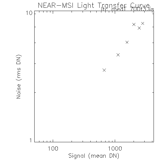
 ltc_medT_700f3.gif (filename of plot; plot made with ltc3.pro)
This is my first LTC plot (above) using the medT data from CCD2 with a filter 700, ND = 1 ( list of images used in plot). There are no "full well" images nor any very low exposure frames (exposures used 200, 350, 500, 650, 800, 917). This range is useful for inspecting the Signal Shot Noise (see also Mikes earlier description of this). I do not know why the 650 exposure does not fall on an otherwise straight line? Calculating a best fit line (excluding the "funny" 650 msec exposure list of images used in fit) I find;
logN(dn) = -0.8639 + 0.4593 logS(dn)Which is sort of close to the rule of 1/2 (see discussion below).
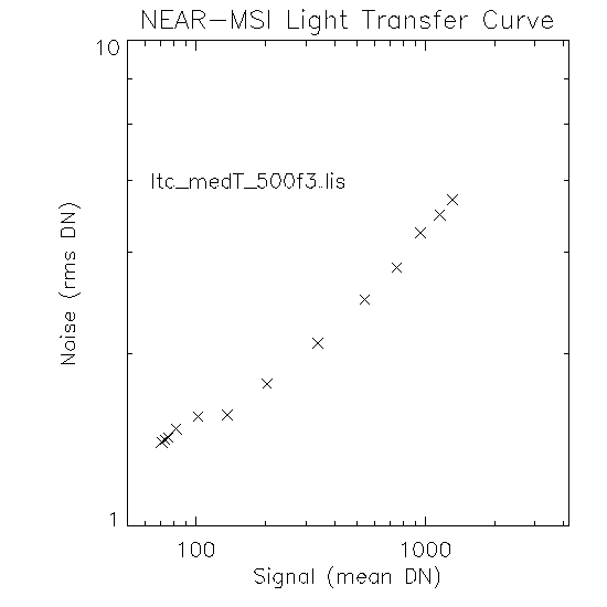 ltc_medT_500f3.gif (filename of plot; plot made with ltc3.pro)
This LTC plot (above) includes short exposure frames as well as long exposure frames (1, 3, 5, 10, 25, 50, 100, 200, 350, 500, 650, 800, 917 msec) all acquired at medium temperature (-31.5 to -33.2), ND = open, filter = 500FS40 ( list of images used in plot). For dark current I used three frames from the "CCD Dark Current Series" taken with an exposure of 500 msec (20580059.FIT, 20580069.FIT, 20580079.FIT). Ok, here we can clearly see the read noise at short exposures that was missing from the previous plot - they kind of bounce around a little, but note the expanded y-scale. However this may be because we have dropped below the readout rate (which I believe is 5 msec), I simply don't know what this would do (help!)? I calculated best fit line to the exposures 200 through 917 msec (Signal Shot Noise portion of the plot) and get this equation (list of images used in equation fit):
logN(dn) = -0.6905 + 0.4011 logS(dn)Apparently this disagrees with mother nature (hope I don't get struck by lightning!)? --------> see discussion below for more details on this. I should mention that I noticed that the temperature was not stable during the measurements.
exposure:temperature

1:-32.0, 3:-31.6, 5:-31.5, 10:-31.5, 25:-31.6,
50:-31.7, 100:-31.8, 200:-32.4, 350:-32.6,
500:-32.9, 650:-33, 800:-33.1, 917:-33.2
Note how the temperature starts at -32.0 then rises to -31.5 and then drops to -33.2 from shortest to longest exposure. Also note the slight swayback nature of the Signal Shot Noise portion of the curve... hmmmmm I wonder if these are related? If I had finished an examination of temperature effects I could probably answer this right off. I guess I better find a test sequence that is more stable, temperature-wise that is!
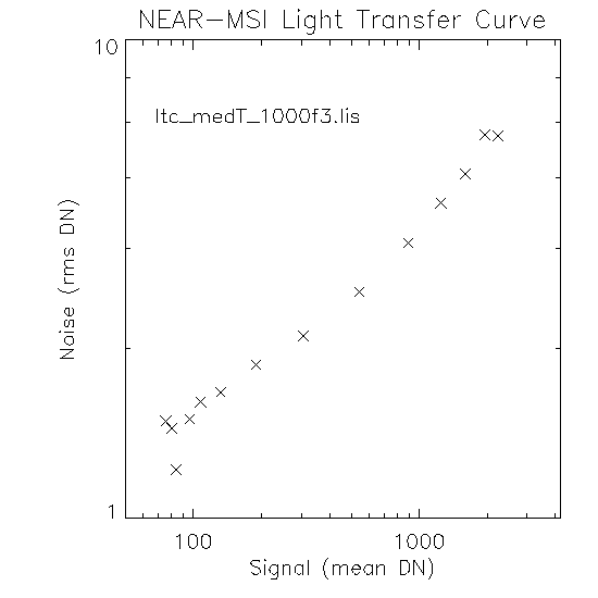 ltc_medT_1000f3.gif (filename of plot; plot made with ltc.pro)
OK, I have plotted another LTC sequence ( above) from the medium temperature sequence with filter = 1000, ND = OPEN ( list of images used in plot). The range of exposure times is the same as the previous plot. Again there is a disagreement (though very close) with the 1/2 slope rule (see discussion below). I calculated the equation below from the data ranging 200 to 800 msec (I excluded the 917 msec beacuse it is "funny" - see plot above). Possibilites: 1) there is something wrong with the sensor, 2) the calb data is labeled improperly, 3) 0.4854 is equivalent to 0.5, I do not the plus/minus of the expected conformance though I suspect it is about +-0.01 (help?), or 4) I screwed up somewhere (I will redo all this and check my code as well as check some other sequences).
logN(dn) = -0.9367 + 0.4854 logS(dn)The same "CCD Dark Current" 500 msec images were subtracted.
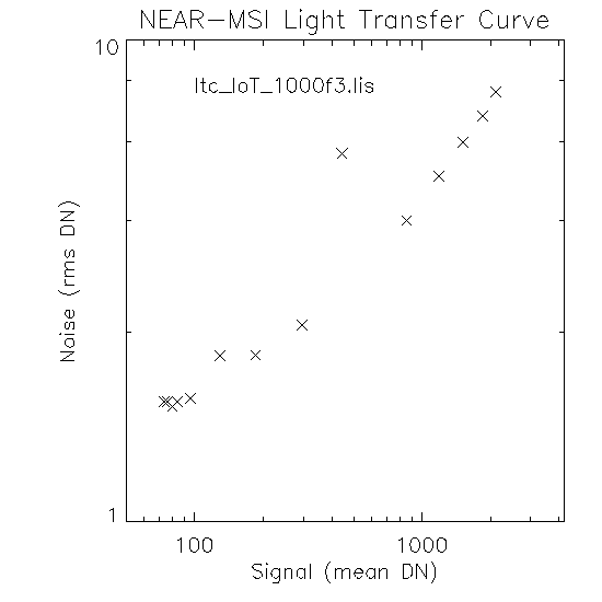 ltc_loT_1000f3.gif (filename of plot; plot made with ltc3.pro)
Here I have plotted another LTC sequence ( above) from the low temperature sequence with filter = 1000, ND = OPEN ( list of images used in plot). These data span the exposure range of 0 - 917 msec, note the spurious data point at the 200 msec exposure (mislabeled???). I calculated a best fit line from 350 - 917 msec and got(list of images used in equation fit):;
logN(dn) = -1.0130 + 0.5079 logS(dn).Again we have a pretty close match to the 1/2 slope rule. As in previous datasets the exposure times fall short of inspecting the full dynamic range of the instrument (dark images used - 20590059.FIT, 20590069.FIT, 20590079.FIT). From this equation I calculate a value for K of 98.7.
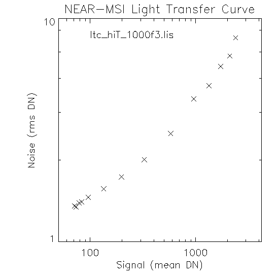 ltc_hiT_1000f3.gif (filename of plot; plot made with ltc3.pro)
Here I have plotted ( above) from the high temperature sequence with filter = 1000, ND = OPEN ( list of images used in plot). The 917 msec point looks "funny" to me (the last point to the right). I have calculated the best fit line twice, once from 200 msec - 917 msec;
logN(dn) = -1.0906 + 0.5380 logS(dn).and again excluding that 917 point;
logN(dn) = -0.9897 + 0.5039 logS(dn).Lets assume the 917 point is bogus and thus we have pretty darn good compliance with the 1/2 rule, from the this equation (the second) I get a value of 92.1 for K (units e-/dn).
N(e) = SQRT(S(e) + R(e)^2) [EQ 1]Where
	N(e) = Total rms noise in terms of electrons
	S(e) = Signal in terms of electrons
	R(e) = Read noise in terms of electrons
The lower portion of the curve is dominated by the read noise of the CCD and camera combination and the upper part by the shot noise of the signal. A number of properties of the CCD (and camera) can be found from the transfer curve:
The lower portion of the curve measures the readout noise floor. The noise floor is dominated by three sources:
TNF = Total Noise Floor SDC = Shot Dark Current CRN = CCD Read NoiseNormally the last two sources are negligible (respectively 0 & 4.5e-) for the case of Space telescope. The total noise floor is typically 15e- or less.TNF = SQRT(CRN^2 + SDC^2 + CRN^2)
The middle portion of the curve characterizes the signal shot noise. On a log-log plot the slope of the light transfer curve is 1/2. This can be shown by using EQ 1 letting R(e) = 0 and taking the log of each side.
N(e) = SQRT(S(e))Therefore,
LogN(e) = 1/2 LogS(e)This characteristic is very valuable when checking out a CCD or camera for the first time. A slope different than 1/2 indicates that you are not agreeing with "Mother Nature".
The upper portion of the curve is a measurement of the "full well" capacity of the CCD. Note the signal continues to increase while the noise drops rather suddenly. This would indicate that the pixels within the n x n area are spilling and filling into one another while in the integration mode or during transfer. As shown this typically occurs at 75,000e- for this device.
When a linear fit is done to the portion of the curve which is signal shot noise limited, the intercept on the signal axis yields the important constant K(e-/DN). This can be shown mathematically from EQ 1.
LET R(e)^2 = 0therefore
N(e) = SQRT(S(e)) [EQ. 2]Converting EQ 2 to DN
N(DN)K = SQRT(S(DN) K) [EQ. 3]Where K is a constant with the units of e-/DN.
N(DN)^2 K^2 = S(DN) KTaking the log of both sides
LogN + LogK = 1/2 Log K + 1/2 Log SWe findLet LogN = 0 or N = 1
LogS = LogK orOnce K is found the entire light transfer curve can be described in units of electrons.K = S which is a remarkable result!
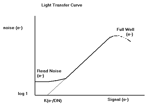 electron.gif (filename of plot; plot sketched with microsft paintbrush)
Also, if the gain of the signal chain and the conversion constant of the A/DC (V/DN) are known, the sensitivity of the (V/e) of the sense node of the capacitance of the CCD can be found.
Si(v/e)=[K(e-/DN) A(v/V) M(DN/V]^-1The notes I have are sort of messy here - I'll have to check that equation.
For example assume that we find K to be 6 e-/DN for a signal chain gain of 84.7 and a A/DC conversion factor of 2^?/2ov=3276DN/V (again messiness needs checking) we find the CCD sensitivity to be .6microvolts/e-.
From the transfer curve the dynamic range for the CCD camera can be easily calculated.
Dynamic Range = (Full Well Signal) / (Readout Noise)Note that I have not run across any full well images yet.
A figure goes hereFor the above transfer curve we find dynamic range to be:
	Dynamic Range = 75,000e-/13e-
		      = 5769
It is possible to find the system constant K by calculating for it as opposed to finding it graphically. Returning to EQ 1.
N(e) = SQRT[S(e) + R(e)^2]Squaring both sides.
N^2(e) = S(e) + R(e)^2Converting to DN.
	K^2N^2 = KS + K^2R^2
	N^2 = (1/K)S + R^2		[EQ. 4]
Way Cool!
Recall
	N = Total Noise (DN)
	R = Read Noise (DN)
	S = Signal (DN)