NOTE ADDED JULY 2005: This page describes a method by which the location of the MER rovers could have been determined, using data from the Mars Relay on Mars Global Surveyor. However, the approach was not needed because the rover team quickly determined where the rovers were located, and this was followed within days by acquisition of Mars Global Surveyor Mars Orbiter Camera images that actually showed the hardware on the surface. The reader of this section should understand that this information has been superseded by actual events.

One of the more important science activities that will be conducted during the first few days that the Mars Exploration Rovers (MERs) are on the surface of Mars will be to determine the exact location of the landing site. Locating the landers is important for a couple of reasons. First, it allows the science team to begin planning where the rover will travel during its 90+ sol mission. Second, it allows scientists to place their findings within a regional and global context provided by orbiter observations.

As part of the Mars Global Surveyor (MGS) Mars Orbiter Camera (MOC) investigation, Malin Space Science Systems (MSSS) will attempt to locate the rovers using data from the MGS Mars Relay (MR) antenna and MOC instrument. These efforts fall into three areas: (1) radiolocation of the landers using doppler measurements performed by the Mars Relay, (2) sightline identification of features seen in MOC high-resolution, narrow angle camera images once a rough location within the landing area has been identified via step 1, and (3) identification of the rover in new, 50-cm/pixel orbiter images acquired during the rover mission.

Radiolocation of the MER Landers using MR Doppler

The Mars Relay (MR) system acquires three doppler measurement every BTTS (16 seconds). During the MGS's pass over the landing site during MER Entry, Descent, and Landing (EDL), when the MER is communicating to the MR, only about 4 or 5 BTTS's will be recorded, or perhaps 12-15 doppler measurements. To analyse the doppler measurements, Scott Davis of MSSS devised a simple process: for each time along the MGS orbit where a doppler measurement is made, he calculates what the doppler signal would be from each longitude, latitude, and altitude within the landing ellipse if that location were in fact the actual location of the lander. He then compares these synthetic values with the actual value measured at that time by the MR. Figure 1 shows a typical MGS early-morning orbit pass by the MER-A landing site in Gusev Crater

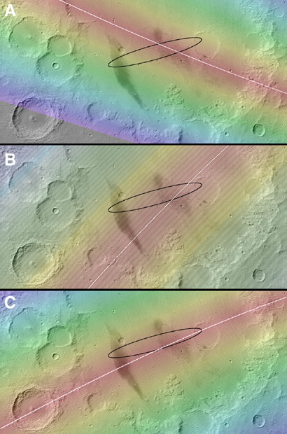
Figure 2 shows single-location maps of the differences between the synthetic and "actual" values (generated in a test of the system) for three times when MGS was approaching (A), passing (B), and receding (C) from the landing location. The three examples were taken near the limits of communication (just after contact is established and just before it is lost). Faint gray lines that alternate light and dark indicate contours of values offset from their neighbors by 256. The white lines are the locus of points along which the minium differences occur--the lander lies somewhere along each white line.

As with the common phenomenon of parallax (look at a object close to you with one eye closed, then open that eye and close the other... the object shifts position in your field of view because of the separation between your two eyes), multiple doppler measurements provide additional information than any single measurement alone. Figure 3 shows how the three separate measurments shown in Figure 2 can be used to locate the lander... it is at the intersection of the three loci of possible locations. The uncertaintly at this point is probably not as good as the lines imply; in reality, the lines are a kilometer or more wide (this is a function of the location prediction for the MGS orbiter and the precision with which the doppler frequency is being measured). On the basis of these data, however, we could with high confidence say (in this test case) that the landing occurred in the eastern half of the ellipse, and probably south of the center-line.

The MGS MOC has two early opportunities to use radiolocation to find each MER lander. The first comes on the day of landing, during the entry, descent, and landing (EDL) pass. Because the rover is expected to communicate with MGS only for about 80-85 seconds (at most) before touching down, doppler measurements will be limited by two factors: first, the MR only takes 3 measurements per 16-second BTTS, so only 12-15 measurements will be made during EDL. Second, since the orbiter only moves about 300 km in this time, the "parallax angle" between these measurements will be small, so there will be more ambiguity in the location. Figurer 4 shows what a 15 measurement location map might look like.

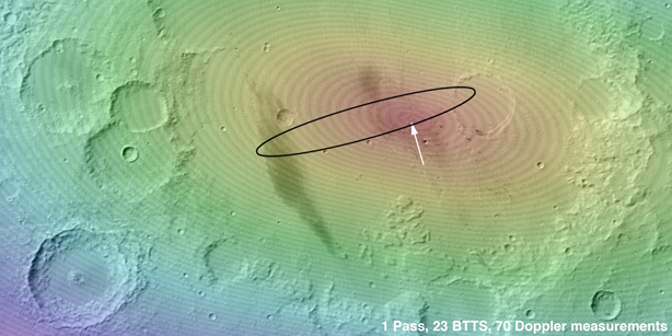
A much better opportunity occurs about 12 hours later, during the first MGS "AM" pass. At this time, the lander will communicate with the orbiter for 6 to 10 minutes (later passes may last as long as 20 minutes). In a 6-minute pass, almost 70 doppler measurements will be made, greatly increasing the "parallax" angle and reducing by statistical averaging errors resulting from frequency sampling. An example of a Sol 2, 2 AM pass doppler map is shown in Figure 5. Location precision is probably better than 1 km and depends mostly on MGS spacecraft location prediction (which have been good to several 100 meters). About a day or two after landing, the MGS tracking data will be available and a refined location will be calculated.

Sightline Analyses: Matching Horizon Features with Features seen from Orbit

From the radiolocation analysis described above, we will have a good place to start looking for features to match between early panorama images taken within the first few sols of surface activity and orbiter images taken before landing. This process is pretty straight forward in areas where good relief is visible, but in areas of very low relief or homogenous morphology (every place looks the same), sight-line analysis can be complicated or even defeated. Below we show an example of sightline analysis for the 1997 lander, Mars Pathfinder.

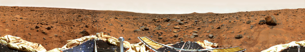
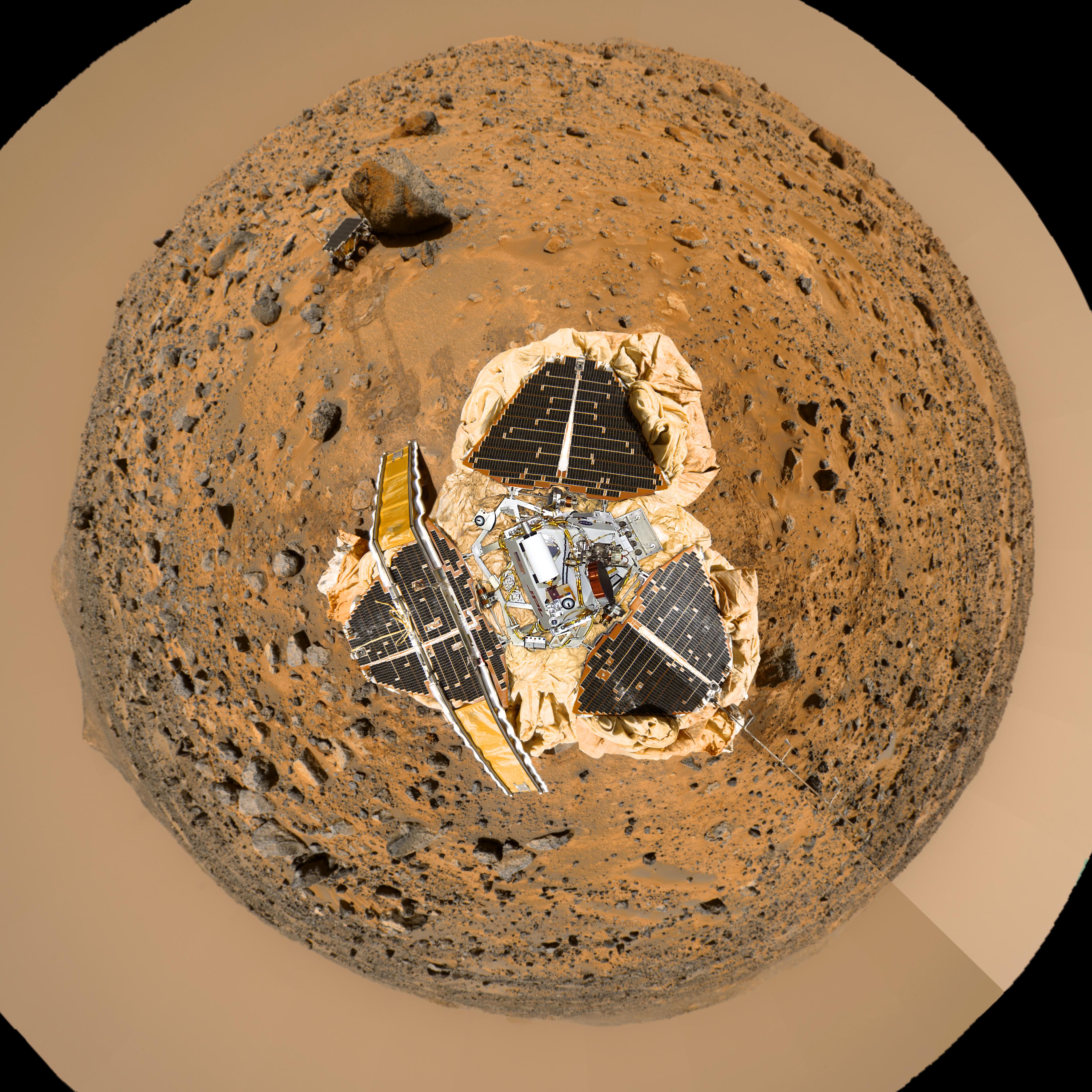
One begins with a parorama view of the landing site. Figure 6 is a pan taken by the Imager for Mars Pathfinder (IMP) early in the Pathfinder mission. Figure 7 shows a stereographic reprojection of that mosaic, which simulates an overhead perspective. In this view, it is easy to see and draw sight-lines between the center of the lander and horizon and sub-horizon features.

By placing the stereographic projection of the lander mosaic with sight-lines on top of a similarly-projected MOC image, one can move the lander mosaic around until sightlines match the overhead morphology. Figure 8 shows this match for the Pathfinder site.

This process has been used for Pathfinder before. The results from analyses before our most recent effort (see below) can be seen at URL http://www.msss.com/mars_images/moc/1_24_00_pathfinder/.

---

Imaging the Landers: Using Image Motion Compensation to get Higher Resolution

Image Motion Compensation

Working with the MGS Spacecraft Team at Lockheed Martin, and MGS Project management and mission planning at the Jet Propulsion Laboratory (JPL), a new imaging technique for improving MOC high resolution images has been devised using the technique of image motion compensation, or IMC. IMC changes the spacecraft pointing at an angular rate comparable to the spacecraft orbital motion to allow the MOC line to dwell longer on a given portion of the planet. This improves the signal to noise ratio (SNR) and, by changing the sampling rate, the spatial resolution in the downtrack direction (the crosstrack direction is fixed by the nature of the detector in the narrow angle camera). Here's how it works:

At a nominal altitude of 400 km, and for a nominal orbital period of 117 minutes, the orbital speed of the spacecraft is about 3.4 km/sec. If the spacecraft didn't rotate in pitch, the nadir would only point towards the planet at one point in the orbit, so the spacecraft rotates at a rate of 360° in 117 minutes, or 0.9 mrad/sec. Projocted at the surface from 400 km altitude, this is equivalent to a reduction in the orbital rate of just over 0.3 km/sec, yielding a ground speed of 3.04 km/sec.

Under normal operations, MOC images must account for these combined motions. As a line-scan system, each line of a MOC image must be exposed and read out before the next line can be taken. If the line time is longer than the equivalent resolution (the "instantaneous" field of view-IFOV--or projected pixel size), then the image resolution is degraded. If the line time is shorter than the equivalent resolution, then the image resolution can be increased in the down-track direction. The cross-track dimension is always equivalent to the IFOV. At a ground speed of 3.04 km/sec and for a projected pixel size of just under 1.5 m/pixel (3.7E-01 IFOV * 400 km), the line time is 1.5 m/3050 m/sec ~ 0.48 msec. This is essentially the fastest line time that the MOC can take images, because it was designed to get square pixels and take as much time as it could per line in order to get the best SNR it could.

By pitching the spacecraft faster than it needs to just maintain nadir orientation, the "effective" ground speed can be reduced by a proportionally larger amount than the 0.3 km/sec required for nadir pointing. Figure 9 shows the relationship between rotation rate in mrad/sec and the equivalent spatial sampling at the MOC's nominal line rater of 0.48 msec/line. At 5 mrad/sec, the sampling scale is about 70 cm/pixel, at 6 mrad/sec it is 50 cm/pixel, and at 7 mrad/sec, the sampling is 30 cm/pixel. MOC resolution is limited by diffraction at about 70 cm/pixel. However, the 2005 Mars Reconnaissance Orbiter (MRO) High Resolution Imaging Science Experiment (HiRISE) experiment is predicated on using internal image motion compensation to provide sampling at smaller scales than its diffraction limit and using image processing techniques to improve the resolution; these same techniques can be employed on MOC images taken at sampling scales smaller than 70 cm. In addition, rather than keeping the sampling rate at 0.48 msec/line, we can increase the line time to collect more photons, thus increasing our signal-to-noise (SNR). A practical compromise between sampling and SNR is to maintain a ground sampling distance of 50 cm (oversampling the MOC diffraction point spread function) and increasing the line time by a factor of 3 (this improves SNR by 3^½, or 1.73).

Figure 9: Relationship between Ground Sampling and IMC S/C Motion

The "down" side to IMC images is that more lines must be taken to cover a specific distance on the ground (in practice, we're taking 3 times the number of pixels). The MOC is limited in the size of images it can take to the size of its buffer, about 80 Mbits. Realtime (40 Mbps) lossless compression helps, but IMC images generally cover much less ground than normal MOC high resolution images.

Another issue that must be addressed is that of planetary rotation. Figure 10 shows the impact of planetary rotation on the shape of the area covered by an image as the effective spacecraft ground speed is reduced by pitch IMC. The high distortion works to reduce the improvements gained by higher sampling. To counteract this effect, the Spacecraft Team devised an approach to include planetary rotation compensation as well as spacecraft velocity compensation.

Figure 10: Image footprint distortion caused by planetary rotation for different amounts of spacecraft velocity compensation. 7.66 mr/sec is the compromise value most recently used in IMC test imaging.

IMC Lander Imaging Test: Pathfinder

So, does this work? To find out, we have taken a small number of test images, including of the Viking 1 and Pathfinder landing sites. Figure 11 shows a comparison of enlargements of the best view of the Pathfinder site taken without IMC and with the new, IMC image. You'll have to look at the large version, the differences are really at the pixel-level. Three effects are noticable in the right-hand (new, IMC) image:

• The SNR is better (you see less "salt-and-pepper" 1-pixel spots in the image relative to the left-hand image).
• The noise pixels that do occur are physically smaller, making them less noticable.
• The image is higher resolution, as can be seen in looking at the rocks around the crater in the lower left of each image.

Figure 11: Comparison of "normal" MOC high resolution image, taken at roughly 1.4 m/pixel and shown here at 0.6 m/pixel, and "IMC" image taken at a ground sampling distance of 0.5 m/pixel and shown here at 0.6 m/pixel.

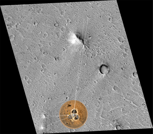
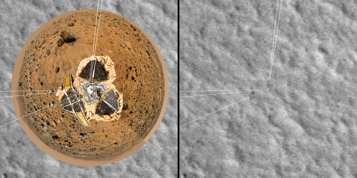
Of course, the proof lies in whether or not we can actually see the Pathfinder lander. Figure 12 shows the lander panorama stereographic projection with sightlines to distant horizon features, and the location at which the sightlines converge. Multi-pixel features at the convergence of the sightlines are interpreted to be the Pathfinder spacecraft and the rock "Yogi" several meters north of the lander.

Figure 12: Enlargement of IMC image of Pathfinder landing site, showing Pathfinder lander at the convergence of optical sightlines to horizon features.

---

© 2003 by Malin Space Science Systems, Inc.