The system gain and read noise characteristics of the NEAR MSI were
determined by computing the photon transfer curve of the instrument.
The photon transfer curve plots the variance of the measured signal
against the derived unbiased signal over a series of increasing
exposures. These points should fall on a line whose slope is equal to
the system gain (in terms of DN / electrons) with a y-intercept equal
to the squared product of the system gain and read noise.
Background
This approach is based on a paper provided by Mark Robinson at USGS.
The original paper is:
Mortara, L. and A. Fowler (1981) Evaluations Of Charge-Coupled Device (CCD) Performance For Astronomical Use. SPIE v. 290, Solid State Imagers for Astronomy, 26-44.
The following is an excerpt from that paper describing the theory behind the approach and the algorithm used to compute the numbers.
The fundamental equation employed is:
V(S) = (G * N)2 + (G * S)
where:
V(S) = variance of the measured signal (units = DN squared)
G = system gain (DN / electrons)
N = r.m.s. system noise (electrons)
S = measured unbiased signal (DN)
Since G and N are constants, this is a linear equation, with the slope equal to G and the y-intercept equal to the square of the product of G and N.
The proof of this equation is as follows:
Assume that the number of electrons observed at pixel i is e(i). Photon statistics implies that variance(e) is equal to mean(e). If P pixels are examined:E(i) = G * e(i) Variance(E) = sum(E(i)2) / P - mean(E)2 = G2 * {sum[e(i)2] / P - mean(e)2} = G2 * variance(e) = G2 * mean(e) = G * mean(E)If noise is given by n(i), then using the same approach as above:Variance(measured noise) = G2 * variance(n) = G2 * N2The resultant signal is then given by:S(i) = E(i) + G * n(i) and, mean(S) = mean(E) (since the average of noise vanishes)Provided that the signal and noise are not coherent, the variances add,V(S) = (G2 * N2) + [G * mean(E)] = (G2 * N2) + [G * mean(S)]
Algorithm
Using flat field images taken at various exposure settings, values for
V(S) and S can be computed. A least
squares fit can then be applied to the equation above to find G and N.
The following steps show exactly how the images are formed:
Given M flat and dark images taken at a given exposure setting, compute the average exposure image and average dark image as:The steps described above yield a number for V(S) and mean(S) for the given exposure setting. Repeating this process for multiple exposure times yields a set of points for which a least squares fit can be computed. From this solution, the slope returns the value of G. Once G has been computed, the y-intercept can be used to compute the noise as follows:mean[X(i,j)] = sum[X(i,j)] / M mean[D(i,j)] = sum[D(i,j)] / MDetermine the deviation in each of the original images as:d(i,j) = X(i,j) - mean[X(i,j)]The variance is then calculated from this deviation as:V(S) = sum[d(i,j)2] / [(M-1) * (i * j)]Note that the (M-1) factor in the above equation is a correction to account for the inaccuracy in the computation of the mean image.The final step calculates the observed signal image as the average exposed image minus the average dark current image. Taking the mean of this image yields the mean true signal for this exposure setting. This final step is illustrated in the following equation:
mean(S) = sum{mean[X(i,j) - mean[D(i,j)]} / (i * j)
	y-intercept = G2 * N2
	N = sqrt[y-intercept / (G2)]
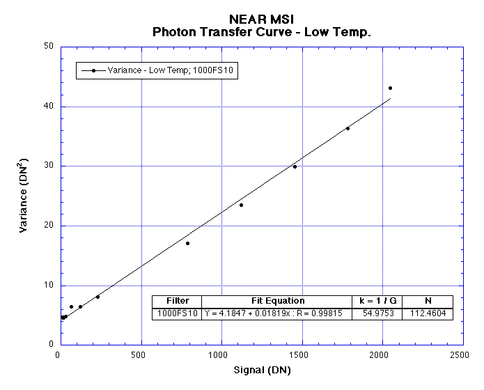
The same images were chosen for this analysis so that the results could be compared with Mark's work. Table 1 lists these images along with the results of the analysis. The following figures show the same results in graphical form:
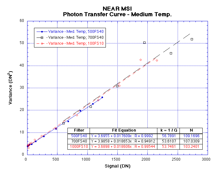
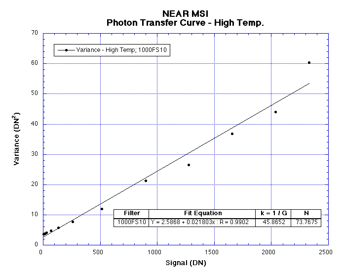
Observations
Note the close correlation between the computed system gain and noise
constants across all of the filters and temperatures that were
examined. The largest deviance is in Figure 3.
Much of this deviation is the result of the single value at the 2400
DN signal level. Discarding that point and recalculating the fit
yields k = 50.6919 and N = 90.1148.
These values are much closer to those calculated at the other
temperatures.
Ignoring the values from Figure 3, the average system gain and noise is given by:
k = 54.7803 electrons / DNN = 107.9753 electrons
The system gain has been reported as k = 1 / G so that the results are in the more familiar units of electrons per DN.
As Mark points out in his memo, if images had been taken at or near the maximum exposure DN, the potential full well of the detector could have been computed. Even with the limited data, however, it is possible to estimate the full-well, and to then compare that value with piecepart measurements made by the manufacturer or during earlier tests at APL. The full well appears to be approximately 225,000 electrons (55 X 4096). If flats are acquired during flight (this will be difficult), it may be worthwhile revisiting this analysis.
Mark Robinson's estimates of system gain were about twice ours. (His stated system noise levels are about 10% of ours, although, in fact, taking the lowest variance levels to be the system noise, his results would have been comparable to ours.) This is curious since, in principal, the methods we use are essentially the same: In effect, Mark divides the equation we use for total measurement variance,
V(S) = (G2 * N2) + (G * mean(S)),
by G2 and then takes its square root, yielding
k*SD = sqrt(N2 + k*mean(S)),
where SD is the standard deviation and where, as before, k = 1/G.
Finally, Mark assumes that the system noise levels are negligible over
some portion of the measurements. (In contrast, we solve directly for
the system noise levels.) With a little rearrangement the equation
then reduces to
SD ~ sqrt(mean(S)/k),
or, taking the logarithm,
log(SD) ~ 1/2 log(mean(S)) - 1/2 log(k).
This is a linear equation in log(SD) and log(mean(S)), with slope 1/2
and y-intercept 1/2 log(k). Mark estimates SD and mean(S) from
measurements, makes a linear fit of log(SD) against log(mean(S)), and
then estimates k as 10 -(y-intercept)/(line slope)
to correct the slope to a value of 1/2.
The discrepancies between Mark's results and ours are due to errors in Mark's implementation of the above equation. First, he accidentally used the mean exposed frame to represent the mean signal; he should have subtracted the mean dark frame. This results in a bias on the order of 60-80 DN in the values of the mean signal.
Second, he erroneously estimates the standard deviation SD. This term should be the root mean square, but he uses the mean of the roots of the squares. That is, he averages the standard deviations where he should have averaged variances and then taken the square root of this. It just so happens that for the case of M=4, if the variances of all the frames are assumed to be the same, these two approaches produce the same values. In general, though, they would differ by a factor of sqrt(4/M).
Finally, he applies a factor of 1/sqrt(1.25) to his (erroneous) RMS estimate to "correct for the increase in noise due to frame subtraction." We take this to mean that he wants to compute an unbiased estimate of the variance, which involves correcting the mean square by M/(M-1), or, equivalently, the RMS by sqrt(M/(M-1)). Mark evidently applies the reciprocal of this term for the case M=5.
The result of the latter two errors for the case M=3 (which most of Mark's estimates use) is roughly a factor of 1.2 in the estimate of the standard deviation, or an offset of about +0.08 in log(SD). The more serious error occurs in estimating the mean signal level due to the dark current bias. This tends to overestimate both the slope and the y-intercept magnitude of the log-log fit.
When these errors are corrected, the log-log method yields results comparable to ours. For example, in the case of the low-temperature measurements using the 1000 nm filter, the log-log method finds k=41.3 electrons/DN using only frames with exposures between 350 and 917 ms, as Mark does. We find k=55.0 electrons/DN using the linear method. Note that, although the discrepancy between our results is much less, some nonetheless remains. This can be traced to the assumption that the system noise levels are negligible over some portion of the measurements:
k*mean(S) >> N2Using our results, we see that for the minimum and maximum mean(S), the above ratio yields:or
N2/(k*mean(S)) << 1
N ~ 100 electronsThus, nowhere over the range of mean(S) is this condition particularly strong. The total RMS noise SD will retain a bias due to N even at the highest values of observed mean(S). This is enough to skew the slope estimate, so that even if the mean signal levels were related to SD as the square root, the log-log slope would not be 1/2. No such bias exists in the method we have used; indeed, the bias is embodied in one of the terms we solve for.
k ~ 50 electrons/DNminimum mean(S) = 5 DN: N2/(k*mean(S)) = 40
maximum mean(S) = 2400 DN: N2/(k*mean(S)) = .08
In summary, since one would have to estimate the system noise term N in order to a posteriori evaluate the validity of the log-log method's assumptions, it would seem simpler to use the linear method from the beginning.