2.1. Landing Site Context
2.2. Science Studies from Descent Imaging
Among the most important questions to be asked about a spacecraft sitting on a
planetary surface is "Where is it?" Radiometric tracking and orbit
determination (both spacecraft-to-Earth and spacecraft-to-spacecraft) and
integration of inertial reference system variations (accelerometers tied to
inertial measurement units) provide answers to this question to varying degrees
of accuracy, but at best can only tell the position to perhaps a few hundred
meters. Surface imaging of features also visible from orbit can be used to
pinpoint lander positions to a few tens of meters or better, provided
that such features are found. However, if the orbiter image resolution is
insufficient to see features visible to the lander, or the local, meter-scale
relief is too great (so the lander cannot see very far), or the surface is
relatively featureless, or the surface has many features but they all look the
same, then the lander cannot be located. The Viking Landers provided good
examples of such circumstances. Through a combination of 20 m/pixel,
relatively low-sun orbiter photography, excellent radiometric tracking from
Earth over a long period of time combined with good inertial position
measurements during landing, and fortuitously landing near craters large enough
to be seen on the horizon in lander images, VL-1 was located to within 50 m[1]. However, despite good
inertial position measurements during landing and good radiometric tracking
data both during the descent and for a number of weeks thereafter, the
homogeneously rugged local relief, nearly featureless horizon, and the lack of
spatially variable landforms in the 40 m/pixel orbiter images defeated all
attempts to determine the location of the VL-2 to better than 10 km.
Why is it important to know "exactly" where a lander is located? The principal
reason is context. It is necessary to determine if the locale is
representative of the region, and, indeed, of the entire planet. It is usually
not possible, just from a lander's perspective, to tell the difference between
what is visible, and what is just over the horizon. The locale may be
anomalous; this must be determined before general interpretations can be made.
Knowing that local meteorology is affected by a nearby escarpment, or that the
lander sits on ejecta from a nearby crater, is important both for local
interpretation, and for extending it farther afield. The context of relating
lander observations to those seen from the orbiter is also important. The
simplest, and most obvious, example is to place surface imaging into the
context of orbiter images (extending and linking crater and boulder
size/frequency relationships, extending surface observations of eolian bedform
wavelength/amplitude/particle size attributes to larger scale, etc.). Other
examples include relating color and/or albedo boundaries seen in orbiter data
down to lander scales (which is particularly difficult to do from the surface
owing to the extremely oblique viewing geometry of the lander instruments), and
providing validation of models used to calculate rock abundance and other
granulometric properties of the surface from thermal emission measurements.
Descent imaging can also provide a context for operations after landing. For
example, the final few images should cover the area around the lander out to 10
meters or more at spatial scales of a centimeter or better. Such images can be
used to plan sampling activities and/or mobility unit traverses, both initially
before lander imaging, and complimentary to those data once they are received.
The easily interpreted, overhead perspective provides such planning activities
considerably greater flexibility, and permits more rapid planning as well.
Advanced techniques in computer graphics and data visualization have been used
to merge lander images with distance measurements, derived from stereoscopic
images or laser rangefinding, in efforts to mimic the overhead perspective.
However, the inability to see surfaces hidden from direct view from the lander
perspective is an essentially fatal flaw in such efforts. The simplest, most
comprehensive way to achieve overhead viewing is from a descent camera.
The scale at which processes modify a planet's surface are dependent on the
vigor of the processes and the timescales over which they act. For Mars, the
vigor of environmental processes has varied with time: recent phenomena appear
to be relatively weak (e.g., wind transport of dust and sand), while ancient
processes appear to have been much more vigorous (e.g., channel formation by
catastrophic flood), although some processes are exceptions to this general
rule (e.g., the occasional contemporary mass movement). Based on cratering
relationships (both the number of craters on surfaces and the degree of
degradation of the ensemble of craters), a crude relationship between size and
age can be formulated: features a few meters across are unlikely to be more
than a few millions of years old, while those hundreds of meters across are
unlikely to be younger than a few hundred of millions of years old. This
relationship suggests that features visible in descent images will cover a
range in ages from hundreds of millions of years to a young as a few years in
age.
JPG = 105 KBytes
GIF = 493 KBytes
Figure 1: Left: Portion of Landsat image showing Antarctic Dry Valleys
at 80 m/pixel. Right: Aerial photograph of area outlined in Landsat image, at
7.5 m/pixel, also indicating location of nested descent images. Note
comparison of landforms at this scale ratio of roughly 10:1.
Relationships between scale and time also occur on Earth, and can be
used to illustrate the study of temporal relationships with descent
images. Figures 2 and Figure 1 shows the relationship between a typical
orbiter image (in this case, a portion of a Landsat frame on the left)
and the first image of a descent sequence (on the right). At a
resolution of about 8 m/pixel and covering an area over 8 km on a
side, the location of the descent image is reasonably visible in the
80 m/pixel orbiter data. The first descent image provides both this
crucial link to the orbiter observations, and the context for all
subsequent frames.
In the specific case of these figures, the increase in resolution from 80
m/pixel to 8 m/pixel spans several important transitions in geomorphic
interpretation. The orbiter data show that the area is mountainous, with
glaciers moving down various topographic gradients. Details of, for example,
the glacial flow cannot be seen at this resolution, but become obvious in the 8
m/pixel data. Note the snout of the Taylor Glacier (lower center, image on
right), which shows ablation pitting along medial streamlines of shear and
morainal debris. Note, too, details of the mountain walls, including mass
movements, and evidence of liquid flow (e.g., small stream channels).

JPG = 115 KBytes
GIF = 597 KBytes
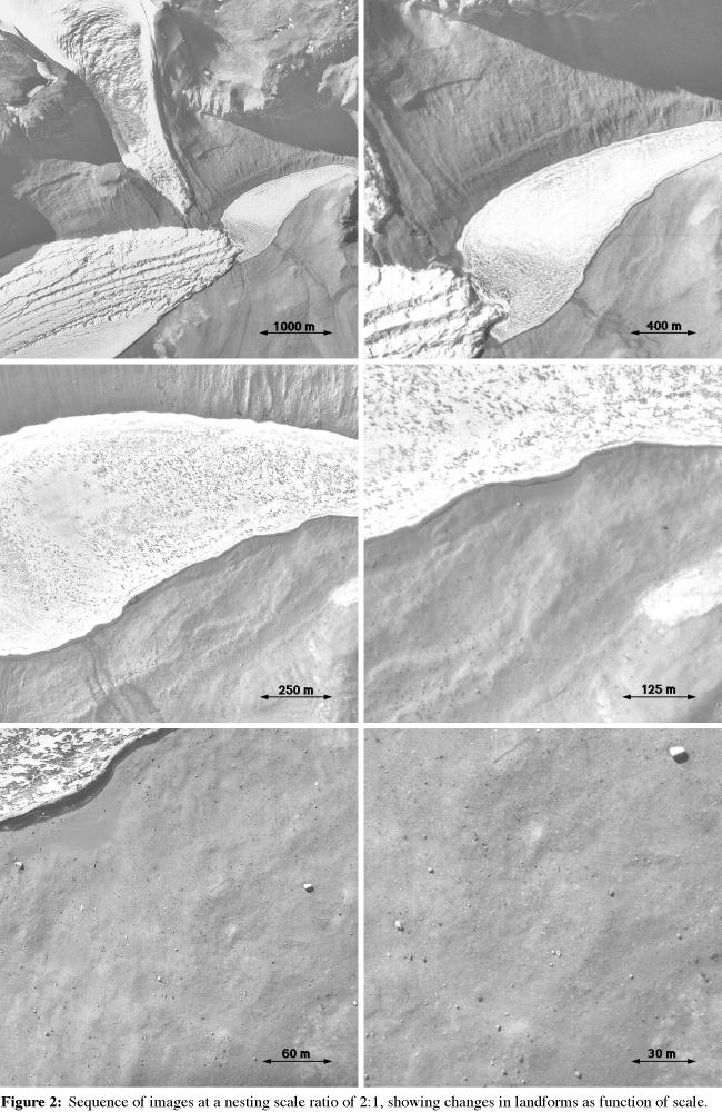
Figure 2: Sequence of images at a nesting scale ratio of 2:1,
showing changes in landforms as a function of scale.
Two "serendipitous" observations, relating to liquid water, can be made using
these images. First, the dark stains in some valley wall- and floor-channels
indicates that liquid water was flowing on the surface in the very recent past.
Indeed, given relatively simple calculations, it is possible to show that the
moisture is only a few weeks old. Second, the dark band around the ice-covered
lake (Lake Bonney, right side, center) can be seen in several of the higher
resolution images to be a liquid water moat. Again, relatively simple
calculations suggest that such moats are ephemeral.
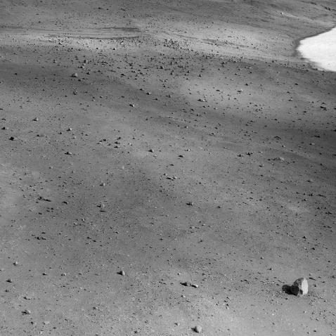
Figure 3 shows an image taken from about 80 m
above the surface, but looking obliquely (the near field is viewed at
an emission angle of 30° , and the far field at about 75° ).
The advantages of oblique viewing, in particular the ability to gain
from a single image some knowledge of subtle relief in the scene and
to provide a more familiar view, are clearly evident in this image.
Note in the lower left foreground a helicopter landing circle
approximately 7 m in diameter.
JPG = 45 KBytes
GIF = 213 KBytes
Figure 3: View of area shown in last two images of Figure 2, showing
advantages of oblique viewing.
One of the more interesting observations that can be made from this
sequence of images is that the scene content varies dramatically with
scale. This is prima facie evidence against the idea
that nature is scale-invariant (i.e., that it isn't
fractal-like). Many geologists have disagreed with the mathematicians
and geophysicists who contend that self-similarity is a fundamental
attribute of geology. Geologists contend that the types and style of
geologic processes and materials clearly vary with scale (i.e., the
mechanisms responsible for breaking individual grains of sand are very
different from those responsible for the shape of river valleys), and
the sequence of images attests to this view. There are clearly
several points in the continuum of scales where the surface takes on
distinctly different properties (the last two frames in Figure 2 are very different from the first two
frames). To the extent that these surfaces reflect different
processes and materials, an analogous sequence on Mars will provide
considerable insight into similarities to and differences with
terrestrial conditions.
 Return to MSSS
Home Page
Return to MSSS
Home Page